App Note 6: Musical Applications of Recursive 2-path Filters

2-path recursive filters are a specific topology of IIR (infinite impulse response) filters with some useful applications in musical digital signal processing. This app note is meant to be a quick overview of the important musical applications of these filters, with lots of links to further reading for details. We also provide open source design functions in Julia.

For interested readers, we can recommend Chapter 11 of “Multirate Signal Processing for Communication Systems” by Fredric J. Harris as a deeper introduction to the topic. This chapter covers a more general class of filters called “Recursive Polyphase Filters”, which allow an arbitrary number of paths, as well as providing a lot of detail on the 2-path case investigated in this app note.

What are 2-path recursive filters?

2-path recursive filters are made up of two real, causal all-pass IIR (infinite impulse response) sub-filters, $H_0(z^2)$ and $H_1(z^2)$ . $H_1(z^2)$ is delayed by one sample and averaged with $H_0(z^2)$ to produce the overall output $H(z)$ . That is, $H(z) = \frac{H_0(z^2) + z^{-1} H_1(z^2)}{2}$ . Graphically, we have:

Since each sub-filter is all-pass, the filtering action comes from constructive and destructive interference of the two paths - frequency regions where they destructively interfere will be attenuated.

The complementary filter

In addition to the main filter $H(z)$ , we can build a complementary filter $H_c(z) = \frac{H_0(z^2) - z^{-1} H_1(z^2)}{2}$ , by subtracting the two paths rather than adding them. This filter is what is called power complementary with the main filter, that is:

|H(z)|^2 + |H_c(z)|^2 = 1

Additionally, the magnitude response of the complementary filter is connected to the main filter by:

|H_c(e^{j\omega})| = |H(e^{\frac{2\pi}{2} - j\omega})|

We provide simple proofs for both of these properties in Appendix 1. Note that for low-pass filters, these properties together tell us that the cutoff frequency must be at $\frac{F_s}{4}$ , and that the response of the passband is fully determined by the response of the stopband (and vice versa).

Application 1: Downsampling

One of the most useful applications of these filters is for efficient anti-aliasing in oversampled systems. Here, oversampling simply means running part of the processing at a higher sampling rate than our final output rate. There are many reasons we might want to do this, for example to reduce aliasing when applying a non-linear effect, or to reduce aliasing when calculating mathematical functions like oscillators.

Oversampled systems are more costly to implement than single-rate systems, firstly because we must run the processing at a higher rate, but also because converting the rates takes computational resources. 2-path recursive filters form an elegant way of efficiently downsampling.

Note from the previous section that the cutoff frequency of these filters is always at $\frac{F_s}{4}$ , where $F_s$ is the sampling rate. This is a natural choice of cut-off for a downsampling filter from 2x the output rate to 1x. If rates higher than 2x are required, we can simply chain these downsampling filters together to achieve any power of two.

In downsampling, we traditionally apply the low-pass filter at the higher rate and then decimate, that is, discard every other sample. The thing that makes these filters particularly efficient for downsampling is that each sub-filter is in terms of $z^2$ , so if we are only looking at every other sample in the output anyways, we can replace each $z^{-2}$ delay element with a $z^{-1}$ delay element and operate at the lower output rate, processing every other sample of the higher input rate. Since there is a high-rate $z^{-1}$ delay element before $H_1$ , this means that $H_0$ will process each even sample and $H_1$ will process each odd sample. This trick is often called the “Noble identity”. Diagrammatically, that is, we have:

Allpass filter structure

So far, we have kept $H_0(z^2)$ and $H_1(z^2)$ fully general all-pass filters. Now that we’re trying to define a filter for a specific application, we’ll actually have to select what types of filters we want to use. We’ll assume that both sub-filters are made up of a cascade of second-order sections of the form $\frac{a + z^{-2}}{1 + az^{-2}}$ . After our Noble Identity trick, these each become first order sections of the form $\frac{a + z^{-1}}{1 + az^{-1}}$ at the lower output rate, which we can realize with the following structure:

Note also that we can share delay elements between multiple sections, for example we can realize $\frac{a_1 + z^{-1}}{1 + a_1z^{-1}}\frac{a_2 + z^{-1}}{1 + a_2z^{-1}}$ like this:

Design procedure

Now that we have our structure in place, all that is left is to choose the coefficients. Of course, this is a very deep topic itself with all sorts of considerations. One choice that is a great match for the oversampling use case is to use an elliptic filter design. The design has been proven to be optimal in the “minimax” sense, that is, it minimizes the maximum signal level over all the frequencies in the stop band. It turns out that musical applications rarely care about this sort of optimality, and rather care more about the total perceptual error over the stop band. However, it’s hard to make precise the exact property to optimize for, and certainly “perceptually optimal” designs would not have a closed-form solution. Elliptic filters are nice in that they create a good response while still having a closed-form solution.

Elliptic filters have four design parameters: the passband ripple, the minimum stopband attenuation, the cut-off frequency, and the order. However, the cut-off frequency must be at $\frac{F_s}{4}$ to match our special structure, and the stopband attenuation determines the passband ripple by our power-complementarity properties. Therefore, only the order and the stopband ripples are truly independent parameters for our application. Note that another property of interest, the transition bandwidth, trades off with the stopband attenuation - for a fixed order, a quieter stopband requires a wider transition band.

The math of elliptic filter design is pretty interesting, but way beyond the scope of this app note. We refer the reader to Richard W. Daniels’ 1974 book “Approximation Methods for Electronic Filter Design”, which has a quite readable treatment. A full design procedure for elliptic coefficients for 2-path filters was presented in “Explicit Formulas for Lattice Wave Digital Filters” by Lajos Gazsi in 1985. In appendix 2, we provide a Julia implementation of the procedure from that paper, giving the coefficients for each section in both paths for a provided order and stopband attenuation. For example, here is the response of a 5th order filter with an -80dB stopband attenuation:

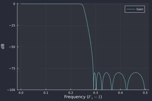
In appendix 3 we provide a short Rust implementation of this filter for reference. The coefficients in the code listing come from the design procedure in appendix 2.

Application 2: Crossovers

Another place where these 2-path filters shine is in crossover filters. Crossover filters are used in multi-band processing, where we want to apply different effects to the “low-frequency” band vs the “high-frequency” band. This is a common technique in mastering and mixing. In general, we want the sum of the two filters to be all-pass so that we get the original spectrum if we don’t do any processing in the two bands.

2-path filters are helpful here because you get a complementary filter “for free” due to the structure - thus, if the main filter is a low-pass and defines the “low-frequency” band, the complementary filter will be high-pass and define the “high-frequency” band. The sum of the two bands will be just $H_0(z^2)$ , which is an all-pass filter.

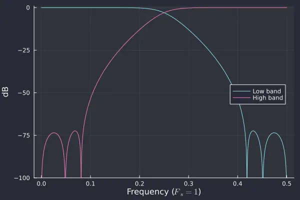
In general, the same elliptic filter design procedure used for downsampling will work well for crossover filters, although we won’t actually decimate the processing, and each delay element will be a two-sample delay. Here’s the crossover response using a 3rd order elliptic filter:

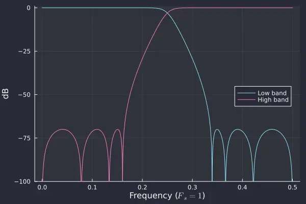
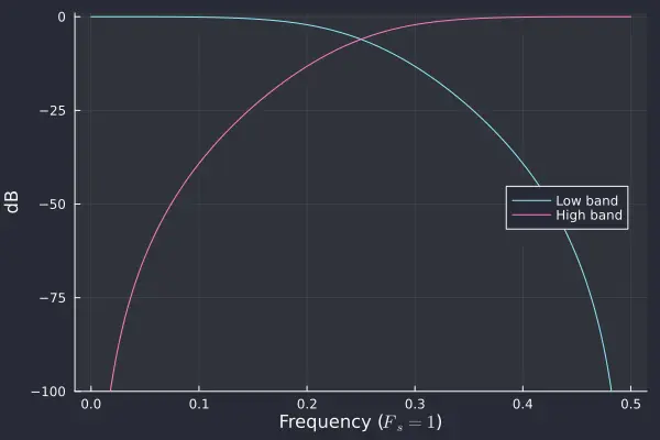
3rd order elliptic filter crossover response

Comparing this to a fourth-order Linkwitz-Riley crossover, we can see that we’ve achieved a much steeper roll-off, meaning better separation between bands. Note that the 3rd order 2-path filter is overall a 7th order filter, since each of the 3 sections is 2nd order, and the delay is first order. Meanwhile, the 4th order Linkwitz-Riley crossover is an 8th order filter since both band filters are 4th order.

4th order Linkwitz-Riley crossover response

Frequency warping

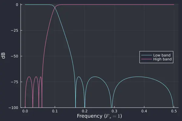
As things stand now, we can only create crossovers at a frequency of $\frac{F_s}{4}$ . Of course, it is often useful to have a controllable crossover frequency. This is no problem since we can use frequency warping (sometimes called a “low-pass to low-pass” transform) to map our crossover frequency to any desired frequency.

Effectively this replaces each delay element with a tuned all-pass filter such that the overall filter is a warped version of the original. We implement this in appendix 2 with the warp_coeffs function. Importantly, after warping $H_0$ and $H_1$ will have $z$ terms, so we will have to implement them as second-order sections with $z^{-1}$ delays (instead of “first-order” sections with $z^{-2}$ delays). Note that the delay before path 1 will also need to be replaced with a warped all-pass filter. Here’s the 3rd order response above warped to a crossover frequency of $\frac{F_s}{10}$ :

$3rd order elliptic filter crossover response warped to a crossover frequency of $\frac{F_s}{10}$$

Perfect reconstruction crossovers

There is a special class of 2-path filters where $H_0(z^2)$ is a pure delay. This class was introduced in “Recursive Nth-Band Digital Filters” by Renfors et al. in 1987, which also provides a design procedure for these filters - they are called “approximately linear phase” designs.

The nice thing about this class is that the sum of the filter and its complement filter is a pure delay, with no phase distortion. That means if you split a signal into two bands, and don’t apply any processing before recombining, you will get a perfect reconstruction of the original signal with no phase distortion.

We implement the design procedure in appendix 2 with the approx_lin_phase_coefficients function. Here’s a frequency response plot of a design with design order 2. This ends up being a 7th order filter overall. Note that the band separation is much worse than the elliptic version of the same order plotted above, but is competitive with the overall 8th order Linkwitz-Riley (LR4) crossover.

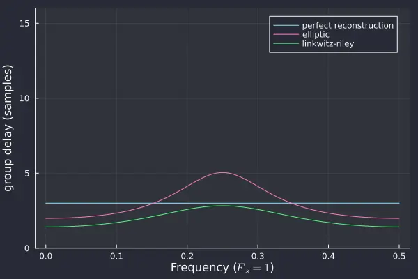
2nd order approximate linear phase crossover response

Here we plot the group delay of the perfect reconstruction version vs the elliptical version, with a crossover frequency of $\frac{F_s}{4}$ , and the overall 8th order Linkwitz-Riley (LR4) crossover. These plots are the sum of the two bands, and express the group delay you’d get from applying the crossover without any processing in the two bands. Note that the perfect reconstruction version indeed has a constant group delay, while the others do not, indicating that some phase distortion is introduced.

Note that if we then apply frequency warping, the crossover will no longer be perfect reconstruction, since the delay elements will be replaced with all-pass filters that do apply some phase distortion. However, the group delay at the crossover frequency will still be less than the elliptical version, since the warping will add distortion to both filters. Here is a comparison of the group delay of the same filters, warped such that the crossover frequency is $\frac{F_s}{10}$ .

group delay comparison of warped filters

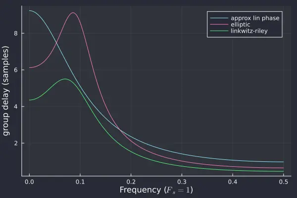
Note that all of the filters have a non-constant group delay, indicating some phase distortion. However, the approximate linear phase version has a monotonic group delay, so at least there are no delay ripples introduced. It’s not clear how beneficial this monotonicity is in practice, but it potentially could reduce transient smearing at the crossover frequency.

Appendix 1: Proofs of properties of the complementary filter

Power complementarity

We show that $|H(z)|^2 + |H_c(z)|^2 = 1$ . This is sometimes called the “Feldtkeller Equation”. This is a simple consequence of the “parallelogram law”, with $A=H_0(z)$ and $B=z^{-1}H_1(z)$ . Then by the parallelogram law $\frac{1}{2}(|A+B|^2 + |A-B|^2) = |A|^2 + |B|^2$ we have

\begin{aligned} |H(z)|^2 + |H_c(z)|^2 &= \frac{1}{2}\left(|H_0(z^2)|^2 + |z^{-1}H_1(z^2)|^2\right) \\ &= \frac{1}{2}(1 + 1) = 1 \end{aligned}

Note that $|H_0(z^2)|^2 = |H_1(z^2)|^2 = 1$ since they are all-pass filters.

Frequency reversal property

Here we show that $|H_c(e^{j\omega})| = |H(e^{\frac{2\pi}{2} - j\omega})|$ . To see this we first expand the definition of $H(e^{\frac{2\pi}{2} - j\omega})$ :

2H(e^{j(\frac{2\pi}{2} - \omega)}) = H_0(e^{j(2\pi - 2\omega)}) + e^{-j(\frac{2\pi}{2} - \omega)} H_1(e^{j(2\pi - 2\omega)})

by Euler’s identities $e^{j\frac{2\pi}{2}} = -1$ , $e^{j2\pi} = 1$

2H(e^{j(\frac{2\pi}{2} - \omega)}) = H_0(e^{j(-2\omega)}) - e^{j\omega} H_1(e^{j(-2\omega)})

Since we assumed $H_0$ and $H_1$ were real filters, they have the well-known property of conjugate symmetry, i.e. $H_0(e^{-j\omega}) = H_0^*(e^{j\omega})$ , which for an all-pass filter means that $H_0(e^{-j\omega}) = \frac{1}{H_0(e^{j\omega})}$ , since for all pass filters conjugates are reciprocals. Thus we have:

\begin{aligned} 2H(e^{j(\frac{2\pi}{2} - \omega)}) &= \frac{1}{H_0(e^{j(2\omega)})} - \frac{e^{j\omega}}{H_1(e^{j(2\omega)})} \\ &= \frac{H_1(e^{j(2\omega)}) - e^{j\omega}H_0(e^{j(2\omega)})}{H_0(e^{j(2\omega)})H_1(e^{j(2\omega)})} \\ &= \frac{-H_0(e^{j(2\omega)}) + e^{-j\omega}H_1(e^{j(2\omega)})}{e^{-j\omega}H_0(e^{j(2\omega)})H_1(e^{j(2\omega)})} \\ &= - \frac{H_0(e^{j(2\omega)}) - e^{-j\omega}H_1(e^{j(2\omega)})}{e^{-j\omega}H_0(e^{j(2\omega)})H_1(e^{j(2\omega)})} \\ &= - \frac{2H_c(e^{j\omega})}{e^{-j\omega}H_0(e^{j(2\omega)})H_1(e^{j(2\omega)})} \end{aligned}

Since $H_1$ and $H_0$ are assumed to be all-pass filters, taking the magnitude of both sides implies $|H(e^{j(\frac{2\pi}{2} - \omega)})| = |H_c(e^{j\omega})|$ as desired.

Appendix 2: Design procedures

using Pkg;
Pkg.activate(".")
Pkg.add("Symbolics")
Pkg.add("Latexify")
Pkg.add("NonlinearSolve")
Pkg.add("Polynomials")
Pkg.add("Plots")
Pkg.add("ForwardDiff")
 
using Symbolics
using Latexify
using NonlinearSolve
using Plots
using Polynomials
using ForwardDiff
theme(:dracula)
set_default(snakecase=false)
 
function elliptic_eps_s(min_stop_attenuation_db)
    sqrt(10 ^ (min_stop_attenuation_db / 10) - 1)
end
 
function elliptic_phi_s(filter_order, min_stop_attenuation_db)
    N = 2 * filter_order + 1
 
    eps_s = elliptic_eps_s(min_stop_attenuation_db)
    eps_p = 1 / eps_s
    r0 = eps_s
    r(ri) = ri ^ 2 + sqrt(ri ^ 4 - 1)
    r1 = r(r0)
    r2 = r(r1)
    x4 = 1/2 * (2* r2) ^ (4/N)
    x(xi) = sqrt(1/2 * (xi + 1/xi))
    x3 = x(x4)
    x2 = x(x3)
    x1 = x(x2)
    x0 = x(x1)
 
    # If following Gazsi, here we choose fs* to be fsmin, which means phi_s* = x0 (normalized f = atan(x0 / pi))
    x0
end
 
function elliptic_w_p(filter_order, min_stop_attenuation_db)
    phi_s = elliptic_phi_s(filter_order, min_stop_attenuation_db)
    w_s = 2 * atan(phi_s)
    pi - w_s
end
 
# The output format will be a tuple of two vectors, each containing the coefficients for each section in each path.
# Coefficients will be all single numbers representing the all-pass coefficient for each section: (1 + aZ^2) / (a + Z^2)
function two_path_elliptic_coefficients(filter_order, min_stop_attenuation_db)
    N = 2 * filter_order + 1
 
    eps_s = elliptic_eps_s(min_stop_attenuation_db)
    eps_p = 1 / eps_s
    phi_s = elliptic_phi_s(filter_order, min_stop_attenuation_db)
    q0 = phi_s
    q(qi) = qi ^ 2 + sqrt(qi ^ 4 - 1)
    q1 = q(q0)
    q2 = q(q1)
    q3 = q(q2)
    q4 = q(q3)
 
    m3 = 1/2 * (2 * q4) ^ (N/2)
    m(mi) = sqrt(1/2 * (mi + 1/mi))
    m2 = m(m3)
    m1 = m(m2)
    m0 = m(m1)
    ms = [m0, m1, m2, m3]
 
    if eps_s / m0 > 1 + 1e-6
        error("Stopband requirements not satisfied: asked for $eps_s, but only got $m0", )
    end
 
    g1 = m0 + sqrt(m0^2 + 1)
    g2 = m1 * g1 + sqrt((m1 * g1)^2 + 1)
    g3 = m2 * g2 + sqrt((m2 * g2)^2 + 1)
    w5 = ((m3 / g3) + sqrt((m3 / g3)^2 + 1)) ^ (1/N)
    w4 = 1 / (2 * q4) * (w5 - 1/w5)
    w3 = 1 / (2 * q3) * (w4 - 1/w4)
    w2 = 1 / (2 * q2) * (w3 - 1/w3)
    w1 = 1 / (2 * q1) * (w2 - 1/w2)
    w0 = 1 / (2 * q0) * (w1 - 1/w1)
 
    c4 = [q4 / sin(i * pi / N) for i in 1:filter_order]
    c3 = 1 / (2 * q3) .* (c4 .+ 1 ./ c4)
    c2 = 1 / (2 * q2) .* (c3 .+ 1 ./ c3)
    c1 = 1 / (2 * q1) .* (c2 .+ 1 ./ c2)
    c0 = 1 / (2 * q0) .* (c1 .+ 1 ./ c1)
 
    gamma = 1 ./ c0
    A = 2 ./ (1 .+ gamma .^2) .* sqrt.(1 .- (q0^2 + 1 / q0^2 .- gamma.^2) .* gamma.^2)
    final_coeffs = -(A .- 2) ./ (A .+ 2)
    # split into even/odd indices to represent the two branches
    (final_coeffs[1:2:end], final_coeffs[2:2:end])
end
 
# Returns a tuple of b, warped_path0, warped_path1. paths is the output of two_path_elliptic_coefficients.
# b is needed to warp the delay in path 1
# warped_pathN is a vector of tuples of section coefficients: (1 + a1Z + a2Z^2) / (a2 + a1Z + Z^2)
function warp_coeffs(paths, cutoff)
    path0, path1 = paths
    b = -(1 - tan(2pi/2 * cutoff)) / (1 + tan(2pi/2 * cutoff))
    function warp_section(a::Number)
        return 2b * (1 + a)/(1 + a * b^2), (b^2 + a) / (1 + a * b^2)
    end
    return b, [warp_section(a) for a in path0], [warp_section(a) for a in path1]
end
 
function approx_lin_phase_coefficients(filter_order, approx_min_stop_attenuation_db)
    # We use expressions from Gazsi's paper to find the passband.
    #
    # Note that we have less attenuation power than elliptical so this won't be quite right.
    # We might want to find a heuristic for setting the attenuation dB (or finding w_p directly)
    w_p = elliptic_w_p(filter_order, approx_min_stop_attenuation_db)
 
    # We use an expression from Renfors paper (claimed to be derived from FIR design with chebyshev polynomials?)
    # to find the attenuation zeros
    # These are the _attenuation_ zeros, that is, the angles for which abs(H(w)) = 1.
    zeros_w = asin.(sin(w_p) .*sin.((1:filter_order) .* pi ./ (2 * filter_order + 1)))
 
    # Now note we may have too many or too few zeros due to numerical noise
    if length(zeros_w) < filter_order
        error("Internal error: Not enough zeros, got $(length(zeros_w))")
    end
 
    zeros_w = zeros_w[1:filter_order]
 
    # phase shift from the linear branch at each zero_w frequency.
    psi = -2 * filter_order .* zeros_w
    Omega = tan.(zeros_w)
 
    # This is the recurrence formula from Henk.
    beta = zeros(filter_order)
    beta_target(i) = tan((psi[i] + zeros_w[i]) / 2)
    beta[1] = beta_target(1) / Omega[1]
    beta[2] = (1 - beta[1] * Omega[2] / beta_target(2)) / (Omega[2] ^2 - Omega[1] ^2)
    function calc_b(r)
        v = beta_target(r)
        v = 1 - beta[1] * Omega[r] / v
        for i in 2:(r - 1)
            v = 1 - beta[i] * (Omega[r]^2 - Omega[i - 1]^2) / v
        end
        return v / (Omega[r]^2 - Omega[r - 1]^2)
    end
    for r in 3:filter_order
        beta[r] = calc_b(r)
    end
    P = zeros(Polynomial{Float64}, filter_order + 1)
    P[1] = Polynomial([1])
    P[2] = Polynomial([1, beta[1]])
    calc_P(r) = P[r-1] + P[r-2] * beta[r - 1] * Polynomial([Omega[r-2]^2, 0, 1])
    for r in 3:(filter_order + 1)
        P[r] = calc_P(r)
    end
 
    # This has given us P, the unfactored polynomial, we need to factor it into roots
    # and then convert the roots into filter sections
    unpaired_roots = Set{ComplexF64}()
    s_sections = []
    for root in roots(P[filter_order + 1])
        # first check if this is a conjugate near a root we already have
        c = conj(root)
        conj_root = nothing
        for existing_root in unpaired_roots
            if abs(c - existing_root) < 1e-6
                conj_root = existing_root
                break
            end
        end
        if conj_root !== nothing
            # we have a conjugate pair, remove it from the set and continue
            delete!(unpaired_roots, conj_root)
            continue
        end
        if abs(imag(root)) < 1e-6
            # we have a real root!
            push!(s_sections, -real(root))
            continue
        end
 
        push!(unpaired_roots, root)
        push!(s_sections, (abs2(root), -2 * real(root)))
    end
 
    # Convert s-section to z-sections
    function convert_section_to_z(term)
        if length(term) == 1
            return (term[1] - 1) / (term[1] + 1)
        end
        if length(term) == 2
            return 2 * (term[1] - 1) / (1 + term[2] + term[1]), (1 - term[2] + term[1]) / (1 + term[2] + term[1])
        end
    end
 
    [convert_section_to_z(root) for root in s_sections]
end

Appendix 3: Rust implementation of downsampling filter

#[derive(Default, Debug, Clone)]
pub struct Downsampler {
    a0: f32,
    a1: f32,
    a2: f32,
    a3: f32,
    b0: f32,
    b1: f32,
    b2: f32,
}
 
impl Downsampler {
    pub fn process(&mut self, input: [f32; 2]) -> f32 {
        let ia0 = input[1];
        let ia1 = (ia0 - self.a1) * 0.061_861_712 + self.a0;
        let ia2 = (ia1 - self.a2) * 0.433_903_75 + self.a1;
        let ia3 = (ia2 - self.a3) * 0.878_088_06 + self.a2;
        self.a0 = ia0;
        self.a1 = ia1;
        self.a2 = ia2;
        self.a3 = ia3;
        let ib0 = input[0];
        let ib1 = (ib0 - self.b1) * 0.223_432_57 + self.b0;
        let ib2 = (ib1 - self.b2) * 0.654_140_25 + self.b1;
        self.b0 = ib0;
        self.b1 = ib1;
        self.b2 = ib2;
        f32::midpoint(ib2, ia3)
    }
 
    pub fn reset(&mut self) {
        *self = Self::default();
    }
}

Appendix 4: Code for the plots in this app note

allpass(a::Number) = Polynomial([1, 0, a]) // Polynomial([a, 0, 1])
allpass(a::Tuple{Number, Number}) = Polynomial([1, a[1], a[2]]) // Polynomial([a[2], a[1], 1])
 
function to_poly_branches(path0, path1, b=0)
    first_branch = prod([allpass(a) for a in path0])
    second_branch = prod([allpass(a) for a in path1]) * Polynomial([1, b]) // Polynomial([b, 1])
    return first_branch, second_branch
end
 
function to_poly_filter(first_branch, second_branch)
    return (first_branch + second_branch)/2
end
 
function to_poly_filter_complement(first_branch, second_branch)
    return (first_branch - second_branch)/2
end
 
# shared x axis
f = range(0, 0.5, length=10000)
w = f * 2pi
 
# First plot: response of elliptic filter
begin
  local ellip_5_0, ellip_5_1 = two_path_elliptic_coefficients(5, 80)
  local ellip_5_0_poly, ellip_5_1_poly = to_poly_branches(ellip_5_0, ellip_5_1)
  local ellip_5_poly_filter = to_poly_filter(ellip_5_0_poly, ellip_5_1_poly)
  local p = plot(ylims=(-100, 1), ylabel="dB", xlabel="Frequency (\$F_s = 1\$)")
  plot!(p, f, 20 * log10.(abs.(ellip_5_poly_filter.(exp.(im * w)))), label="Gain")
  display(p)
  savefig(p, "6/ellip_5.png")
end
 
# We share the 3rd-order response in a few plots
 
ellip_3_0, ellip_3_1 = two_path_elliptic_coefficients(3, 70)
ellip_3_0_poly, ellip_3_1_poly = to_poly_branches(ellip_3_0, ellip_3_1)
ellip_3_poly_filter = to_poly_filter(ellip_3_0_poly, ellip_3_1_poly)
ellip_3_poly_filter_complement = to_poly_filter_complement(ellip_3_0_poly, ellip_3_1_poly)
ellip_3_b, ellip_3_0_warped, ellip_3_1_warped = warp_coeffs((ellip_3_0, ellip_3_1), 0.1)
ellip_3_0_poly_warped, ellip_3_1_poly_warped = to_poly_branches(ellip_3_0_warped, ellip_3_1_warped, ellip_3_b)
ellip_3_poly_filter_warped = to_poly_filter(ellip_3_0_poly_warped, ellip_3_1_poly_warped)
ellip_3_poly_filter_complement_warped = to_poly_filter_complement(ellip_3_0_poly_warped, ellip_3_1_poly_warped)
 
# Second plot: response of crossover
begin
  local p = plot(ylims=(-100, 1), ylabel="dB", xlabel="Frequency (\$F_s = 1\$)")
  plot!(p, f, 20 * log10.(abs.(ellip_3_poly_filter.(exp.(im * w)))), label="Low band", leg=:right)
  plot!(p, f, 20 * log10.(abs.(ellip_3_poly_filter_complement.(exp.(im * w)))), label="High band")
  display(p)
  savefig(p, "6/ellip_3_crossover.png")
end
 
# Define LR4 crossover and warped version
begin
  local q = sqrt(2)/2
  local alpha = 1/2q
 
  butterworth_low = Polynomial([1 / 2, 1, 1 / 2]) // Polynomial([1 - alpha, 0, 1 + alpha])
  lr4_crossover_low = butterworth_low * butterworth_low
  butterworth_high = Polynomial([1 / 2, -1, 1 / 2]) // Polynomial([1 - alpha, 0, 1 + alpha])
  lr4_crossover_high = butterworth_high * butterworth_high
 
  # we just pre-warp z since we don't need to calculate the warped coeffs
  local cutoff = 0.1
  local b = -(1 - tan(2pi/2 * cutoff)) / (1 + tan(2pi/2 * cutoff))
  lr4_crossover_low_warped(z) = lr4_crossover_low((1 + b*z) / (b + z))
  lr4_crossover_high_warped(z) = lr4_crossover_high((1 + b*z) / (b + z))
end
 
# Third plot: comparison of response of LR4 crossover
begin
  local p = plot(ylims=(-100, 1), ylabel="dB", xlabel="Frequency (\$F_s = 1\$)", leg=:right)
  plot!(p, f, 20 * log10.(abs.(lr4_crossover_low.(exp.(im * w)))), label="Low band")
  plot!(p, f, 20 * log10.(abs.(lr4_crossover_high.(exp.(im * w)))), label="High band")
  display(p)
  savefig(p, "6/lr4_crossover.png")
end
 
# Fourth plot: warped response of crossover
begin
    local p = plot(ylims=(-100, 1), ylabel="dB", xlabel="Frequency (\$F_s = 1\$)", leg=:right)
    plot!(p, f, 20 * log10.(abs.(ellip_3_poly_filter_warped.(exp.(im * w)))), label="Low band")
    plot!(p, f, 20 * log10.(abs.(ellip_3_poly_filter_complement_warped.(exp.(im * w)))), label="High band")
    display(p)
    savefig(p, "6/ellip_3_crossover_warped.png")
end
 
allpass_linphase_coeffs(a::Number) = Polynomial([a, 0, 1]) // Polynomial([1, 0, a])
allpass_linphase_coeffs(a::Tuple{Number, Number}) = Polynomial([a[2], 0, a[1], 0, 1]) // Polynomial([1, 0, a[1], 0, a[2]])
 
begin
  local lin_phase_filter_order = 2
  local lin_phase_crossover_coeffs = approx_lin_phase_coefficients(lin_phase_filter_order, 80)
  local lin_phase_lin_branch = (1 // Polynomial([0, 1])) ^ (lin_phase_filter_order * 2 - 1)
  local lin_phase_nonlin_branch = prod([allpass_linphase_coeffs(a) for a in lin_phase_crossover_coeffs])
  lin_phase_low = (lin_phase_lin_branch + lin_phase_nonlin_branch) / 2
  lin_phase_high = (lin_phase_lin_branch - lin_phase_nonlin_branch) / 2
 
  # Note that we don't currently have code to directly warp coefficients, so we just
  # pre-warp z here. It shouldn't be hard to implement this if you want!
  local cutoff = 0.1
  local b = -(1 - tan(2pi/2 * cutoff)) / (1 + tan(2pi/2 * cutoff))
  lin_phase_low_warped(z) = lin_phase_low((1 + b*z) / (b + z))
  lin_phase_high_warped(z) = lin_phase_high((1 + b*z) / (b + z))
end
 
# Fifth plot: response of perfect reconstruction crossover
begin
  local p = plot(ylims=(-100, 1), ylabel="dB", xlabel="Frequency (\$F_s = 1\$)", leg=:right)
  plot!(p, f, 20 * log10.(abs.(lin_phase_low.(exp.(im * w)))), label="Low band")
  plot!(p, f, 20 * log10.(abs.(lin_phase_high.(exp.(im * w)))), label="High band")
  savefig(p, "6/approx_lin_phase_2_crossover.png")
  display(p)
end
 
function group_delay(filt, w)
  phase(w) = imag(log(filt(exp(im * w))))
  group_delay(w) = -ForwardDiff.derivative(phase, w)
  group_delay(w)
end
 
# Sixth plot: group delay comparison
begin
  local p = plot(ylims=(0, 16), ylabel="group delay (samples)", xlabel="Frequency (\$F_s = 1\$)")
  plot!(p, f, group_delay.(lin_phase_low + lin_phase_high, w), label="perfect reconstruction")
  plot!(p, f, group_delay.(ellip_3_poly_filter - ellip_3_poly_filter_complement, w), label="elliptic")
  plot!(p, f, group_delay.(lr4_crossover_low + lr4_crossover_high, w), label="linkwitz-riley")
  savefig(p, "6/group_delay_comparison.png")
  display(p)
end
 
# Seventh plot: warped group delay comparison
begin
  local p = plot(ylabel="group delay (samples)", xlabel="Frequency (\$F_s = 1\$)")
  plot!(p, f, -group_delay.(z -> lin_phase_low_warped(z) + lin_phase_high_warped(z), w), label="approx lin phase")
  plot!(p, f, group_delay.(ellip_3_poly_filter_warped - ellip_3_poly_filter_complement_warped, w), label="elliptic")
  plot!(p, f, -group_delay.(z -> lr4_crossover_low_warped(z) + lr4_crossover_high_warped(z), w), label="linkwitz-riley")
  savefig(p, "6/group_delay_comparison_warped.png")
  display(p)
end

5: Continuous-time Convolution Anti-aliasing for Ring Modulation