App Note 4: Analysis of Roland single-transistor VCA
This is an analysis of a single-transistor VCA design found in a few roland products such as the TR-909 (e.g., for the snare drum volume control), and the JX-8P (for the oscillator mixing section). Similar designs were used by Korg in the MS20 and the Poly-61. I’m not sure who implemented this design first, I’d be very interested to hear from anyone who knows more about the history of this design.
This app note assumes some knowledge of analog circuits and may not fully explain some prerequisites. If you find this confusing, please improve it by contributing a PR!
This design is interesting in that it uses a transistor in saturation mode, which is a rather unusual operating mode for a bipolar transistor in analog electronics. It also has a rather startlingly low component count for a VCA!
The design
Let’s look at a simplified diagram of the circuit (component values here taken from JX-8P):
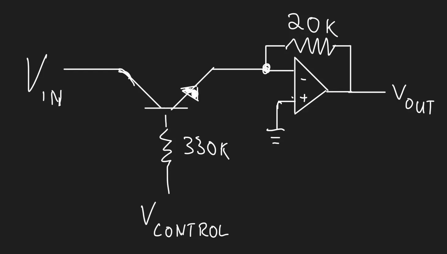
In this design, varies from to , and varies from to .
Using ohm’s law, we note that where is the emitter current.
Assuming an ideal op-amp, we note that the voltage at the non-inverting input of the op-amp is , since it is equal to the voltage at the inverting input.
Thus, to understand the behavior of the circuit, we can analyze a simpler circuit
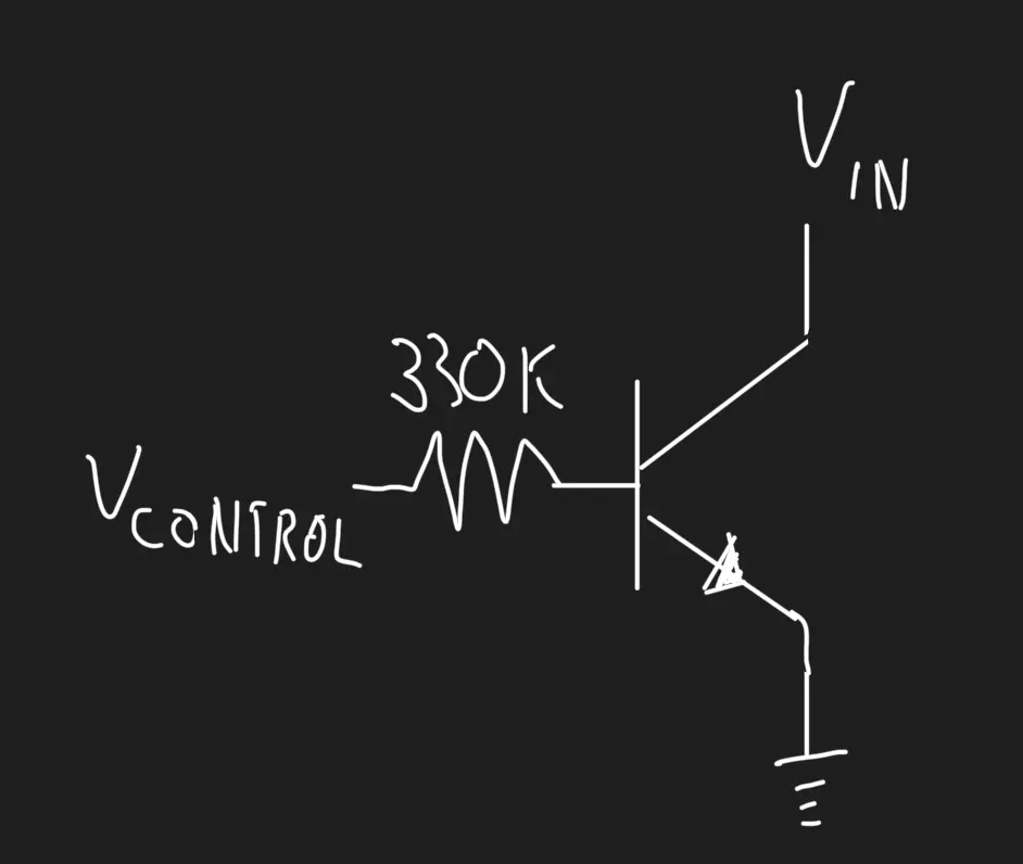
The “output” of this simplified circuit is the emitter current.
Note from ohm’s law, , where is the 330k base resistor.
Analysis with Ebers-Moll
One interesting thing to note in this configuration is that the Base voltage is going to be higher than both the emitter and collector voltages. This puts the transistor in the so-called “saturation” region, where a lot of the really simple transistor models for hand calculations don’t apply. We’ll go back to the Ebers-Moll model, which is a simple yet general purpose model that works in all regions. Wikipedia has a good reference for this model. From wikipedia:
Here , , , and are all transistor parameters (saturation current, thermal voltage, forward current gain, and reverse current gain respectively).
Initial Approximations
We now apply some approximations. First we make use of the fact that for most transistors. Applying this to the above equations we have:
Now, we make use of the fact that in the saturation region, . Now,
does not depend on
Our next step is to recall that is actually related to by ohm’s law, i.e., . This means that our first approximation becomes
But by definition, so
Now, we note that , so
We see now that , at least in this approximation, is only a function of not . This means, when considering the behavior under small changes, we can treat as a constant.
as a function of
We now turn our attention to the output, . First we recall that , so since is ground, we have . So, our approximation for becomes
or, re-arranging,
Note that since is small, this is approximately linear in .
The intuition here is that since is constant, increasing will increase , which will increase , since . Increasing will cause more current to flow through the emitter, due to the diode action of the base-emitter junction.
as a function of
Since we don’t want to work with the cumbersome Lambert’s W function, we can make a somewhat crude approximation that . This lets us make progress on this analysis. We’ll confirm that this approximation gives qualitatively correct behavior with SPICE simulations later. Given this assumption, we have:
re-arranging,
applying log to both sides,
Full approximation
Finally, we can plug in our approximations for and together:
simplifying,
so we see, that this is indeed approximately a multiplication of and .
Spice simulations
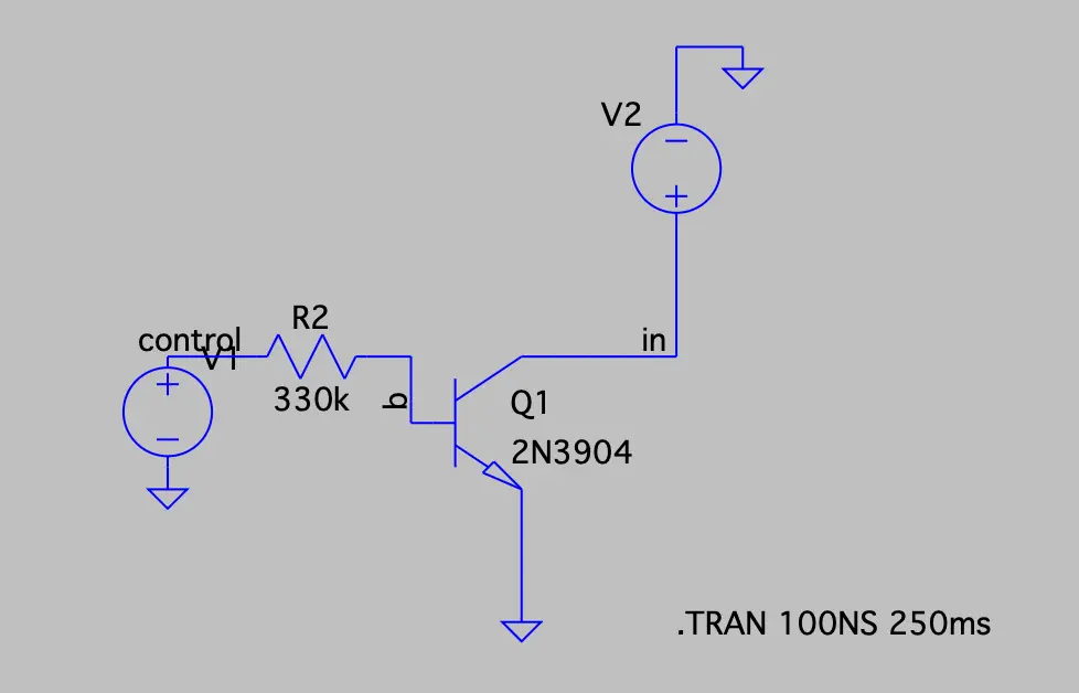
Here we verify the behavior of the circuit with an LTSpice simulation. (download)
The circuit we’re simulating is the simplified circuit above.
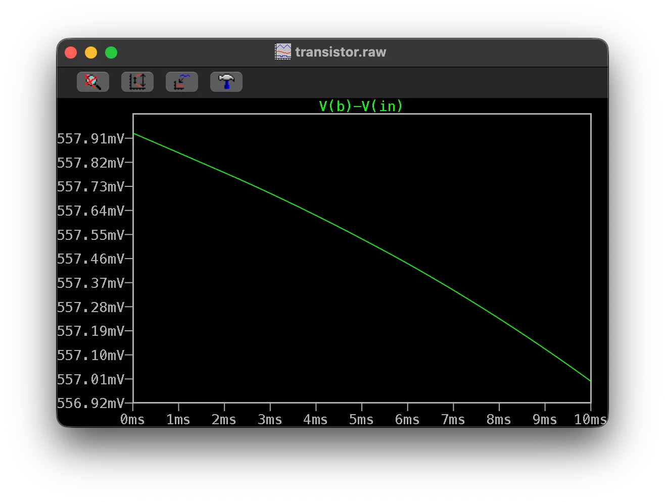
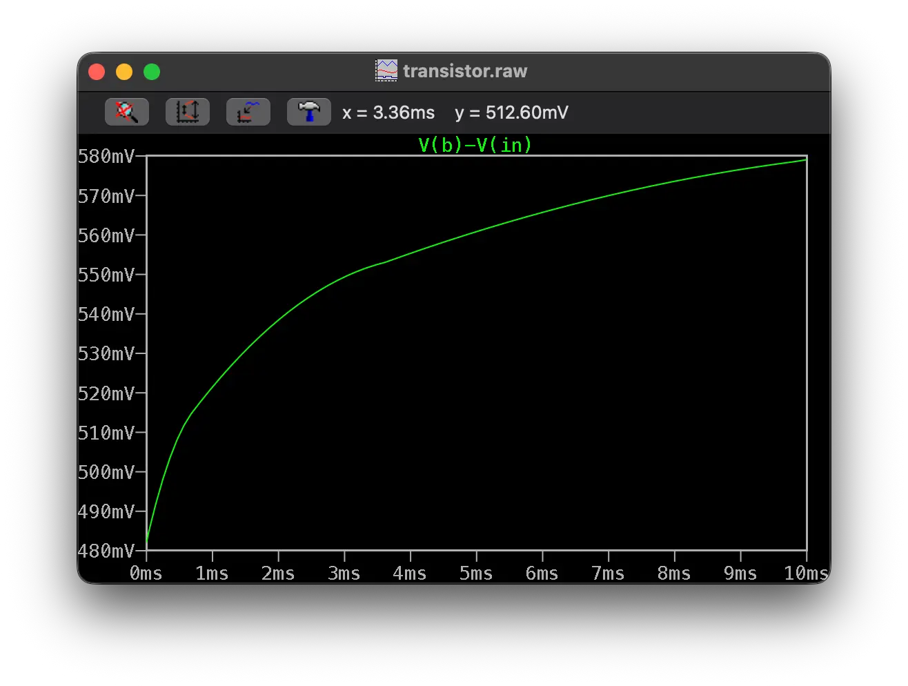
We can use this simulation to verify a few key points of the analysis above. First, we fix at and sweep from to . We can see that only varies from to , so indeed it’s a good approximation to treat as independent of .
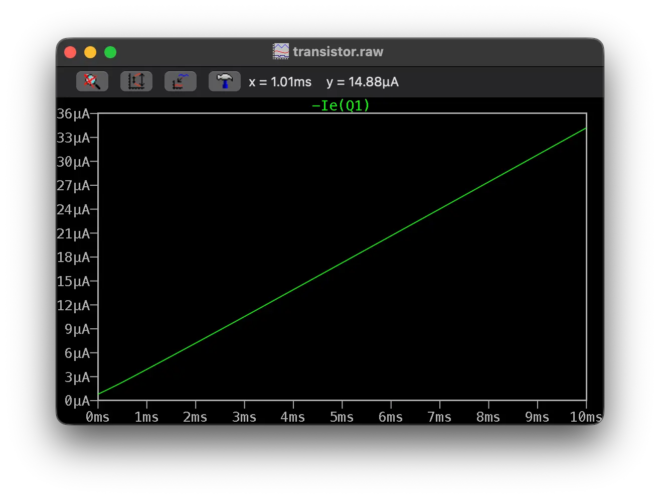
Now, let’s check the dependence of on . We keep at and sweep from to . We see that indeed looks like a small slice of an exponential function (and approximately linear), a great match to the by-hand analysis above.
We can also check the dependence of on . To do this, we keep at and sweep from to . We see that indeed looks something like a logarithmic function of .
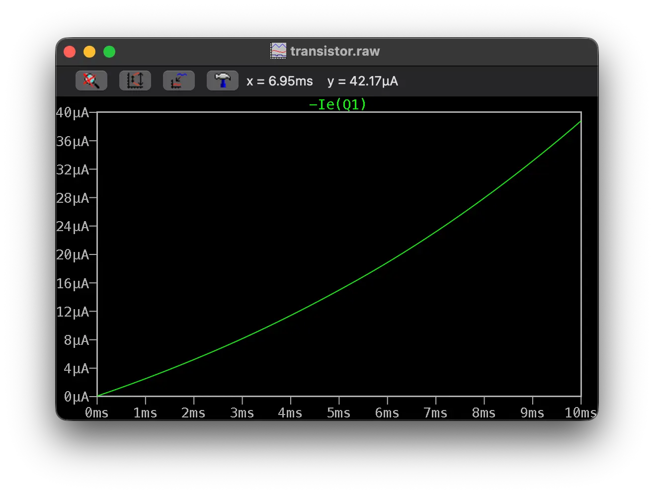
Let’s check the dependence of on . We again keep at and sweep from to . Here we have what appears to be a linear dependence between and , as predicted above.
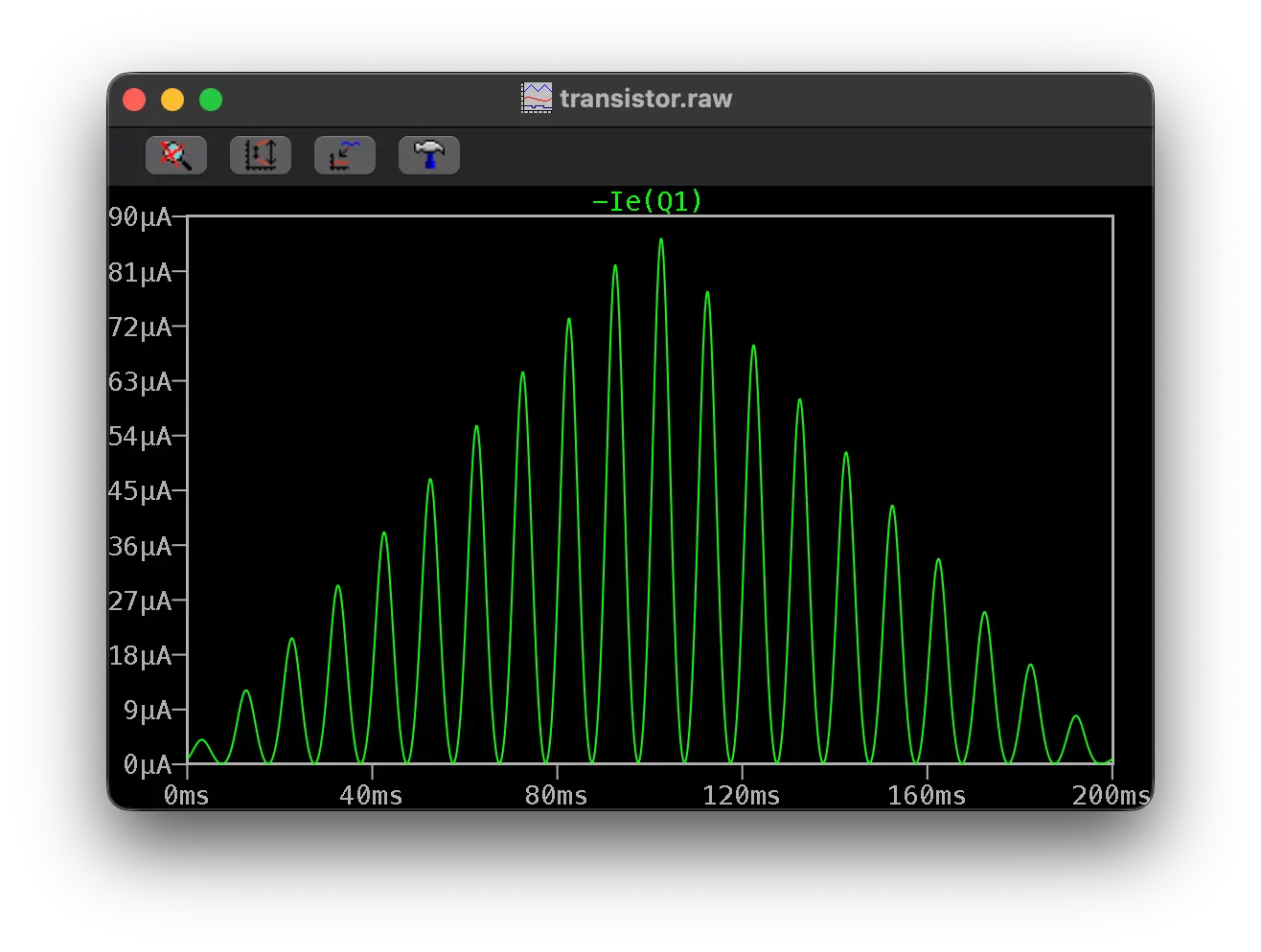
Finally, let’s do a full simulation of the VCA action of circuit. We apply a sine wave with peaks at and at a frequency of 100hz to and sweep from to and back to to . We see that the output matches the predicted behavior of a multiplication of the two signals.
Downsides of this design
Wow, these simulations look pretty good! Given that this design only needs a single transistor, why isn’t it more popular? A couple reasons come to mind:
- Thermal noise. Given that an exponential function is applied to , the level has to be very low to approximate linearity. In Roland’s implementation, peak to peak voltage is kept under . This means that the effective noise floor is quite high at most real-world temperatures.
- Non-linearity. Even with a signal as low as , we have some visible non-linearity in (see spice simulations). Linearity of looks pretty good, though. It might be interesting to reverse the inputs and apply the signal through the “control” input of the circuit.
- The design depends on the transistor being deep in saturation mode, which means that the control voltage must be significantly above both the emitter voltage and the input voltage at the collector. This means that careful control of bias is required.
- The design is very dependent on the temperature, since the term is temperature dependent.