App Note 3: Quick Derivation of BLIT, BLEP, BLAMP polynomials

This is a lightning-round, no-frills derivation of polynomial BLIT, BLEP, and BLAMP functions. I hope to expand this into a more didactic treatment in the future, but for now this will probably be most useful as a reference for those who have some experience with these functions.

BLIT

BLIT stands for “band limited impulse train”. The “train” part indicates that we are interested in synthesizing a repeated waveform signal that will be made up of many discontinuities; however in this note we only consider a single pulse at time $t = 0$ . As a pedantic terminology clarification, in most implementations, the band-limiting is only approximate, so some sources call this “quasi-band-limited”. However, in this note we will just use “band-limited” to mean “approximately band-limited”, which matches most of the literature.

A band-limited impulse is a continuous signal that has the following properties:

It must be at least approximately band-limited
Sampling it must yield approximately a sampled impulse (i.e., a sampled signal with a single non-zero sample at time $t = 0$ )

The only signal that meets both of these requirements exactly (rather than approximately) is the Sinc function, which has the downside of being infinitely long, so is never used in practice. See “Splitting the Unit Delay” by Laasko et al for more details and various approximation schemes that don’t involve infinite-length signals.

In this App Note, we’ll focus on a specific family of polynomial band-limited impulses called Lagrange polynomials. For a given order $N$ , we can construct a polynomial with support $1 + N$ . Here, support means the duration of signal that is non-zero. These are often called “polyBLIT”.

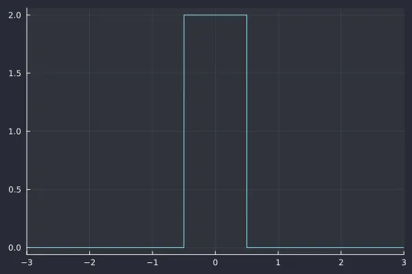
0th order polyBLIT

The simplest one is order 0, which has support 1.

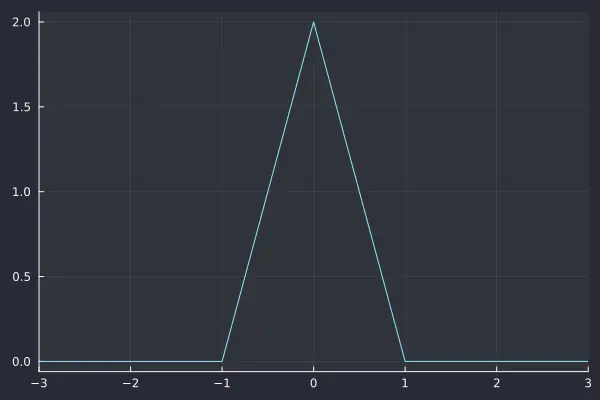
\text{polyBLIT}_0(t) = \begin{cases} 2 & \text{if } t \in \left[-\frac{1}{2}, \frac{1}{2}\right] \\ 0 & \text{otherwise} \end{cases}

0-order polyBLIT

1st order polyBLIT

Order 1 is just a linear interpolation kernel, with support 2.

\text{polyBLIT}_1(t) = \begin{cases} 2t + 2 & \text{if } t \in \left[-1, 0\right) \\ -2t + 2 & \text{if } t \in \left[0, 1\right] \\ 0 & \text{otherwise} \end{cases}

1-order polyBLIT

Order 2 and above are not treated here, but it’s a quadratic lagrange polynomial. More information is available on Wikipedia.

BLEP

“BLEP” stands for “Band Limited Step”. It represents the integral of a band-limited impulse. Generally we “package” these functions as residuals, with the 0-order step function subtracted off. This packaging makes applications a lot more convenient - we can generate our waveform without any consideration for anti-aliasing, then add the residual to each signal discontinuity to easily reduce the aliasing caused by the discontinuity.

When using a BLEP to anti-alias a discontinuity, you must scale it by the size of the “jump” at the discontinuity. The BLEPs derived in this note are normalized for a jump from -1 to 1 (total distance of 2), for example the discontinuity of a downward-going saw wave or the upward-going discontinuity of a square wave. For bigger or smaller jumps, you must scale the BLEP linearly with the size of the jump.

To construct a BLEP, we need to start with a band-limited impulse, and then integrate it. polyBLITs of order $N$ will integrate into a so-called “polyBLEP” with order $N+1$ .

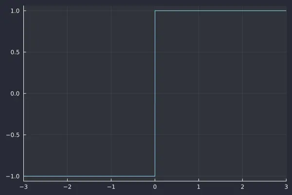
0th order polyBLEP

Note that a polyBLEP of order 0 is simply the 0-order step function, and has no residual (as an aside, I guess this makes the dirac delta in some sense an “order -1” polyBLIT, since you can integrate it into a 0-order polyBLEP).

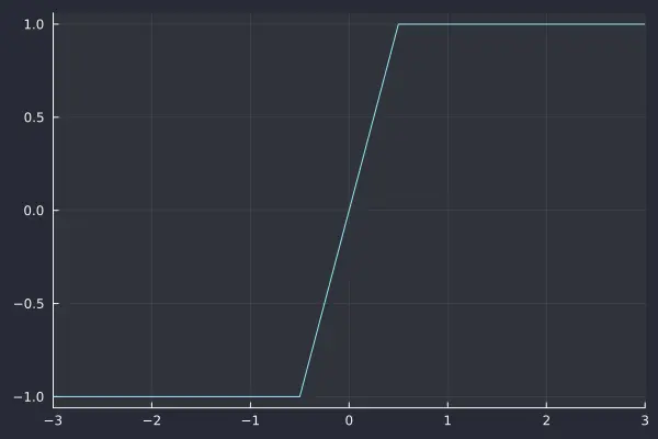
\text{polyBLEP}_0(t) = \begin{cases} -1 & \text{if } t \lt 0 \\ 1 & \text{otherwise} \end{cases}

0-order polyBLEP

1st order polyBLEP

To derive the 1-order polyBLEP, we need to integrate the 0-order polyBLIT, which we can do piecewise. Since each segment is a polynomial, we can integrate it using the power rule:

\text{polyBLEP}_1(t) = \begin{cases} -1 & \text{if } t \lt -\frac{1}{2} \\ 2t & \text{if } t \in \left[-\frac{1}{2}, \frac{1}{2}\right] \\ 1 & \text{otherwise} \end{cases}

1-order polyBLEP

Now, we can calculate the residual by subtracting out the 0-order step function:

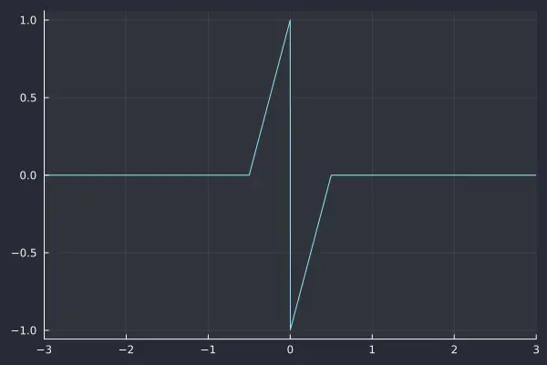
\text{polyBLEP}_1^{\text{residual}}(t) = \begin{cases} 0 & \text{if } t \lt -\frac{1}{2} \\ 2t + 1 & \text{if } t \in \left[-\frac{1}{2}, 0\right) \\ 2t - 1 & \text{if } t \in \left[0, \frac{1}{2}\right] \\ 0 & \text{otherwise} \end{cases}

1-order polyBLEP residual

2nd order polyBLEP

We derive the 2-order polyBLEP by integrating the 1-order polyBLIT, which again can be done piecewise with the power rule.

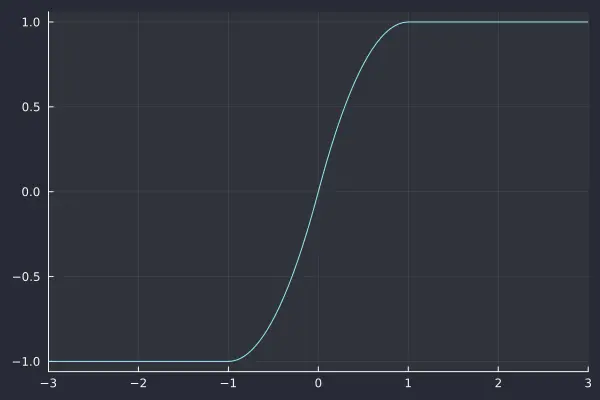
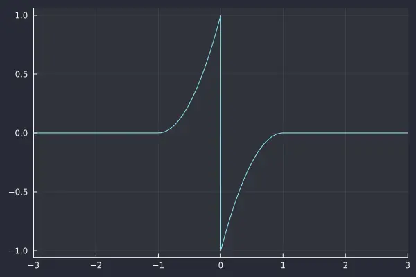
\text{polyBLEP}_2(t) = \begin{cases} -1 & \text{if } t \lt -1 \\ t^2 + 2t & \text{if } t \in \left[-1, 0\right) \\ -t^2 + 2t & \text{if } t \in \left[0, 1\right] \\ 1 & \text{otherwise} \end{cases}

2-order polyBLEP

Now, we can calculate the residual by subtracting out the 0-order step function:

\text{polyBLEP}_2^{\text{residual}}(t) = \begin{cases} 0 & \text{if } t \lt -1 \\ t^2 + 2t + 1 & \text{if } t \in \left[-1, 0\right) \\ -t^2 + 2t - 1 & \text{if } t \in \left[0, 1\right] \\ 0 & \text{otherwise} \end{cases}

simplifying:

\text{polyBLEP}_2^{\text{residual}}(t) = \begin{cases} 0 & \text{if } t \lt -1 \\ (t + 1)^2 & \text{if } t \in \left[-1, 0\right) \\ -(t - 1)^2 & \text{if } t \in \left[0, 1\right] \\ 0 & \text{otherwise} \end{cases}

2-order polyBLEP residual

BLAMP

“BLAMP” stands for “Band Limited Ramp”. It represents the integral of a BLEP. Similar to BLEPs, these are most often “packaged” as residuals, with the absolute value function (i.e., the 1st order ramp function) subtracted off. This gives a signal that can be added to any derivative discontinuity to easily reduce the aliasing caused by it. Most often these are used for triangle waves.

One important usage note is that, similar to BLEPs, the BLAMP needs to be scaled by the size of the derivative “jump”. The BLAMPs derived in this note are normalized for a jump of derivative from -1 to 1.

There is no meaningful 0-order BLAMP, since the lowest order where it’s possible to have a derivative discontinuity is 1.

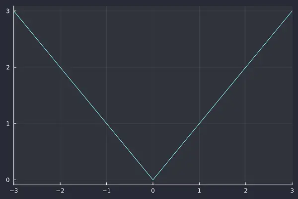
1st order BLAMP

The 1st order BLAMP is simply the 1st order ramp function or the absolute value function, and it has no residual.

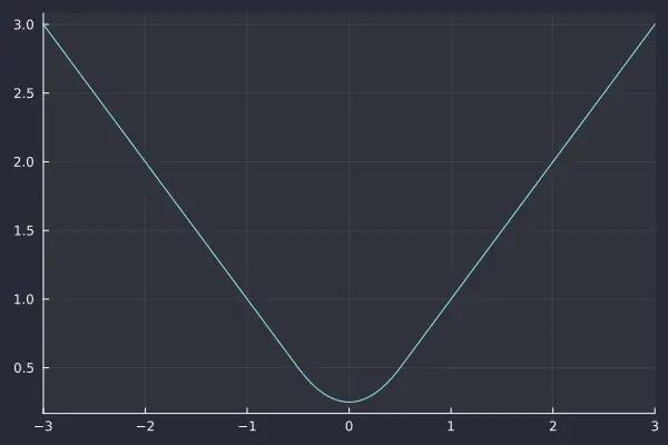
\text{polyBLAMP}_1(t) = \begin{cases} -t & \text{if } t \lt 0 \\ t & \text{otherwise} \end{cases}

1-order polyBLAMP

2nd order BLAMP

The 2nd order BLAMP is the integral of the 1st order BLEP, and like other derivations this is done piecewise with the power rule.

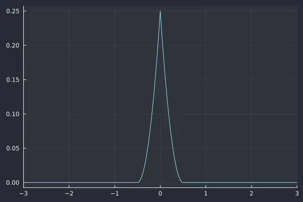
\text{polyBLAMP}_2(t) = \begin{cases} -t & \text{if } t \lt -\frac{1}{2} \\ t^2 + \frac{1}{4} & \text{if } t \in \left[-\frac{1}{2}, \frac{1}{2}\right] \\ t & \text{otherwise} \end{cases}

2-order polyBLAMP

Now, we can calculate the residual by subtracting out the 1st order ramp function:

\text{polyBLAMP}_2^{\text{residual}}(t) = \begin{cases} 0 & \text{if } t \lt -\frac{1}{2} \\ t^2 + t + \frac{1}{4} & \text{if } t \in \left[-\frac{1}{2}, 0\right) \\ t^2 - t + \frac{1}{4} & \text{if } t \in \left[0, \frac{1}{2}\right] \\ 0 & \text{otherwise} \end{cases}

simplifying:

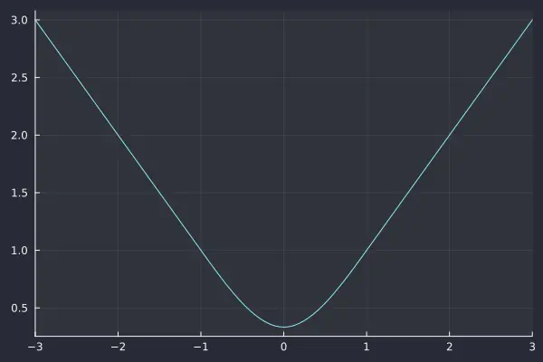
\text{polyBLAMP}_2^{\text{residual}}(t) = \begin{cases} 0 & \text{if } t \lt -\frac{1}{2} \\ (t + \frac{1}{2})^2 & \text{if } t \in \left[-\frac{1}{2}, 0\right) \\ (t - \frac{1}{2})^2 & \text{if } t \in \left[0, \frac{1}{2}\right] \\ 0 & \text{otherwise} \end{cases}

2-order polyBLAMP residual

3rd order BLAMP

In exactly the same way as the 2nd order BLAMP, we can integrate the 2nd order polyBLEP to get the 3rd order BLAMP.

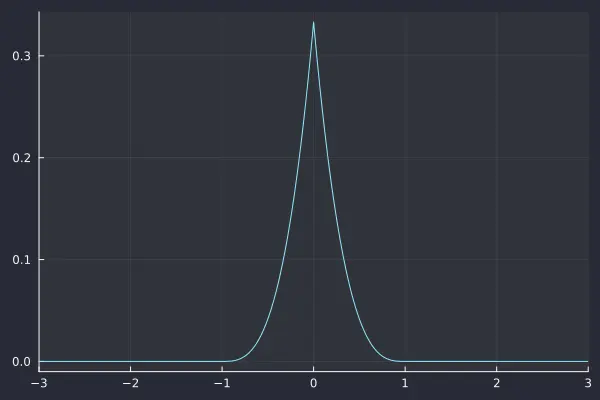
\text{polyBLAMP}_3(t) = \begin{cases} -t & \text{if } t \lt -1 \\ \frac{1}{3}t^3 + t^2 + \frac{1}{3} & \text{if } t \in \left[-1, 0\right) \\ -\frac{1}{3}t^3 + t^2 + \frac{1}{3} & \text{if } t \in \left[0, 1\right] \\ t & \text{otherwise} \end{cases}

3-order polyBLAMP

Again, we can calculate the residual by subtracting out the 1st order ramp function:

\text{polyBLAMP}_3^{\text{residual}}(t) = \begin{cases} 0 & \text{if } t \lt -1 \\ \frac{1}{3}t^3 + t^2 + t + \frac{1}{3} & \text{if } t \in \left[-1, 0\right) \\ -\frac{1}{3}t^3 + t^2 - t + \frac{1}{3} & \text{if } t \in \left[0, 1\right] \\ 0 & \text{otherwise} \end{cases}

3-order polyBLAMP residual

Higher order BLAMPs are not treated here, but their derivation follows the exact same pattern of integrating a polyBLEP, which in turn was derived by integrating a polyBLIT.

Higher-order discontinuity residuals

To summarize, we’ve created residuals for:

signal discontinuities (BLEP residuals)
first derivative discontinuities (BLAMP residuals)

No applications immediately come to mind; but you can continue this pattern to create residuals for discontinuities of higher order derivatives, by integrating BLAMPs. I’m not aware of a name for these higher-order residuals. This note won’t explicitly derive these, but the technique should be clear.

An alternate derivation

Another way to derive the same equations for low-order BLITs, BLEPs and BLAMPs is to consider a naive impulse, step, or ramp respectively, then convolve it with a continuous filter multiple times.

To derive the polynomial family above, the filter that we apply is a box filter, or what we called the 0th order polyBLIT above. Convolving with this filter raises the polynomial order by 1 each time we apply it.

In this alternative derivation, to derive a polyBLIT of a given order $N$ , we start with the dirac delta function, and apply the box filter $N + 1$ times. To derive a polyBLEP of order $N$ , we start with the step function (0th order polyBLEP above), and apply the box filter $N$ times. To derive a polyBLAMP of order $N$ , we start with the 1st order ramp function (1st order polyBLAMP above), and apply the box filter $N - 1$ times.

This derivation gives a nice signal-processing way to think about these BLITs, BLEPs and BLAMPs, since they are derived simply by applying filters repeatedly. This makes it easier to analyze the properties of these functions, since we can use all the tools of filter analysis. Additionally, we can imagine swapping out the box filter with other “root” filters to get a different family of BLITs, BLEPs and BLAMPs.

However, for signals derived from polyBLITs of order 2 and above (which are not treated in this note), the two derivation techniques start to diverge! This is because an order-2 lagrange polynomial is not the same as applying the box filter twice to a dirac delta.

References

“Alias-Free Digital Synthesis of Classic Analog Waveforms” by Stilson and Smith, ICMC 1996, contains an early treatment of the BLIT approach (using windowed sinc kernels)
“Splitting the Unit Delay” by Laasko, Välimäki, Karjalainen, and Laine, IEEE Magazine 1996, is a review of fractional-delay filters, which overlap a lot in design techniques with BLITs.
“Hard Sync Without Aliasing” by Brandt, 2001, contains an early treatment of the BLEP approach (pre-integrated BLEPs)

Appendix: Code for figures

using Pkg;
Pkg.activate(".")
Pkg.add("Symbolics")
Pkg.add("Plots")
using Symbolics
using Plots
theme(:dracula)
 
@variables x y
 
function save_plot(filename, eq)
    savefig(plot(eq, xlims=(-3, 3), legend=false), filename)
end
 
save_plot("polyblit-0.png", ifelse(x < -0.5, 0, ifelse(x <= 0.5, 2, 0)))
save_plot("polyblit-1.png", ifelse(x < -1, 0, ifelse(x <= 0, 2 * (x + 1), ifelse(x <= 1, 2 * (1 - x) , 0))))
save_plot("polyblep-0.png", ifelse(x < 0, -1, 1))
save_plot("polyblep-1.png", ifelse(x < -0.5, -1, ifelse(x <= 0.5, x * 2, 1)))
save_plot("polyblep-1-residual.png", ifelse(x < -0.5, 0, ifelse(x <= 0, x * 2 + 1, ifelse(x <= 0.5, x * 2 - 1, 0))))
save_plot("polyblep-2.png", ifelse(x < -1, -1, ifelse(x <= 0,  x * x + 2 * x, ifelse(x <= 1, 2 * x - x * x, 1))))
save_plot("polyblep-2-residual.png", ifelse(x < -1, 0, ifelse(x <= 0, x * x + 2 * x + 1, ifelse(x <= 1, 2 * x - x * x - 1, 0))))
save_plot("polyblamp-1.png", ifelse(x < 0, -x, x))
save_plot("polyblamp-2.png", ifelse(x < -0.5, -x, ifelse(x <= 0.5, x ^ 2 + 0.25, x)))
save_plot("polyblamp-2-residual.png", ifelse(x < -0.5, 0, ifelse(x <= 0.0, x ^ 2  + x + 0.25, ifelse(x <= 0.5, x ^ 2 - x + 0.25, 0))))
save_plot("polyblamp-3.png", ifelse(x < -1, -x, ifelse(x <= 0,  1/3 * x ^ 3 + x ^ 2 + 1/3, ifelse(x <= 1, x ^ 2 - 1/3 * x ^ 3 + 1/3, x))))
save_plot("polyblamp-3-residual.png", ifelse(x < -1, 0, ifelse(x <= 0,  1/3 * x ^ 3 + x ^ 2 + x + 1/3, ifelse(x <= 1, x ^ 2 - 1/3 * x ^ 3 - x + 1/3, 0))))

2: Modeling LFOs for BBD Chorus