App Note 1: Parameterized Exponential Scaling Functions

When providing continuous controls to users in the form of knobs or sliders, it’s often useful to scale these parameters non-linearly so that moving the control changes the parameter in a way that “feels” natural. Clearly, this is more art than science, but there’s still mathematics involved! This brief application note defines one type of non-linear mapping that’s often useful as a control scaling.

Setting Up the Problem

To set up the problem, let’s consider parameters and UI elements that are both defined for intervals $[0, 1]$. We can define the “scaling function” as a continuous function $f$ from the interval of the UI element (the knob or slider) to the interval of the underlying parameter.

The simplest mapping function is the identity function. $f(x) = x$.

Generally we’ll want $f$ to have a few propertiers:

• It should be invertible, that is, there should exist a function $g$ from the underlying parameter to the UI interval such that $g(f(x)) = x$ and $f(g(x)) = x$ for all $x \in [0, 1]$
• It should be monotonic, i.e., for all $y > x$ in the interval, $f(y) > f(x)$

We can see that these two properties together imply a couple of other facts:

• $f(0) = 0$
• $f(1) = 1$

Clearly, our simple identity function satisfies all these properties!

Exponential mappings

The exponential function is truly magnificent. As we’ll see, we can use it to build a family of scaling functions. These scaling functions can be intuitive for a lot domains, because they act as a mathematically simple approximation to the way some of our senses work (e.g., pitch or loudness in audio).

We can define a scaling function based on the exponential function by setting a few parameters ($a$, $b$, $c$):

However, the properties of scaling functions restrict our choices a little: we can see that the requirement that $f(0) = 0$ implies that $b = 1$, and the requirement that $f(1) = 1$ implies $\exp(a) = c + b = c + 1$, which we can also express as $a = \log(c + 1)$. So really, we have only one “free” parameter to choose, $c$. Simplifying while recalling that $\exp(\log(z)x) = z^x$ by definition, we have

We can see that for positive $c$, this is clearly monotonic and it has an inverse $g(x) = \log_{c + 1}(cx + 1)$, so it’s a totally valid scaling function!

Choosing $c$ with set points

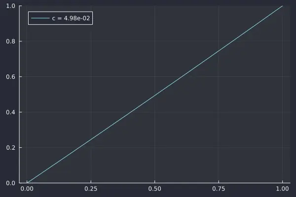
How should we pick $c$? Well, like everything else in the business of choosing scaling functions, it’s a matter of taste! As we lower $c$, we’ll get closer and closer to the identity mapping, and as we raise $c$, we’ll get curvier and curvier, eventually staying near 0 until the very end of the range.

One way we might want to choose $c$ is if we have specific points we want to map, i.e., $p, q \in (0, 1)$ such that $f(p) = q$. Clearly we must have $p > q$ due to the shape of possible exponential maps. This gives us an equation we can solve to select $c$, $q = \frac{(c + 1)^p - 1}{c}$, which we can simplify to $qc + 1 = (c + 1)^p$. For reasons that will be convenient later, we can rewrite this to $(qc + 1)^{\frac{1}{p}} = c + 1$, or

Unfortunately, this is a transcendental equation, which requires tricks to solve analytically (often involving the W function). I don’t know of any tricks that help with this one, unfortunately! Please let us know if you have a way to solve this in closed form for general $p$!

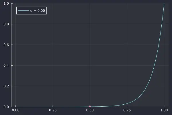
Fixing $p$ to solve the equation

One way to make progress is by fix $p = \frac{1}{2}$, this becomes a quadratic equation that’s easy to solve!

$(qc + 1) ^ 2 - c - 1 = q^2c^2 + (2q - 1)c = 0$ $q^2c + 2q - 1 = 0$ $c = \frac{1 - 2q}{q^2}$

Let’s plot this!

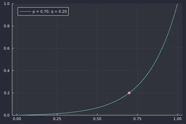
Varying $p$

This is very cool, but we didn’t want $p$ to be fixed at a set value like $0.5$ — rather, we want to be able to set $p$ to any value in the interval! How can we achieve this? Well, it’s difficult or impossible to find an analytic solution, but it’s quite tractible to solve the equation above for general $p$ numerically on a computer!

One classic technique for numerical solutions is called the Newton-Raphson method. This is a great, simple technique that can solve a wide class of equations, which our equation $(qc + 1)^{\frac{1}{p}} - c - 1 = 0$ is almost in. There is one issue, in that $c = 0$ will be a solution for all $p$! This isn’t good because in the expression for $f$, we divide by $c$, so we’re assuming $c > 0$. One way to fix this in practice is to multiply both sides by $\frac{1}{c}$, which will cause Newton’s method to avoid this spurious solution. That is, we’re solving:

A super-simple way to implement newton’s method is by calculating the derivative with dual numbers, however going into the implementation is out of scope for this brief note! Please check out the code in the appendix for more!

Using Newton-Raphson, we can indeed define $c$ to match arbitrary $p$ and $q$!

Appendix

Below is the code used to make the plots!

import Pkg
Pkg.activate(".")
Pkg.add("Plots")
using Plots
using Printf
theme(:dracula)
 
r = range(-3, 20, length=100)
anim = @animate for logc in vcat(r, reverse(r))
    p = plot(ylimits = (0, 1))
    c = exp(logc)
    i = range(0.0, 1.0, length=1000)
    plot!(p[1], i, ((c + 1) .^ i .- 1.) ./ c, label=(@sprintf "c = %.2e" c))
end
gif(anim, "changingc.gif")

r = range(0.001, 0.499, length=100)
anim = @animate for q in vcat(r, reverse(r))
    p = plot(ylimits = (0, 1))
    c = (1 - 2 * q) / (q * q)
    i = range(0.0, 1.0, length=1000)
    plot!(p[1], i, ((c + 1) .^ i .- 1.) ./ c, label=(@sprintf "q = %.2f" q))
    scatter!(p[1], [0.5], [q], label="")
end
gif(anim, "fixedp.gif")

Pkg.add("DualNumbers")
using DualNumbers
 
function plot_circ(x, y, r, name)
    anim = @animate for phi in range(0, 2 * pi - 0.01, length=100)
        pl = plot(ylimits = (0, 1))
        p = cos(phi) * r + x
        q = sin(phi) * r + y
 
        guess =  (1 - 2 * q) / (q * q)
        if abs(guess) < 1e-10
            guess = 1
        end
        tries = 0
        function evalGuess(x)
            return ((q * x + 1) ^ (1 / p) - x - 1) / x
        end
        while (tries < 100 && abs(evalGuess(guess)) > 1e-8)
            d = Dual(guess, 1)
            attempt = ((q * d + 1) ^ (1 / p) - d - 1) / d
            guess -= realpart(attempt) / dualpart(attempt)
            tries += 1
        end
        c = guess
        i = range(0.0, 1.0, length=1000)
        if (abs(c) < 1e-10)
            plot!(pl[1], i, i, label=(@sprintf "p = %.2f, q = %.2f" p q))
        else
            plot!(pl[1], i, ((c + 1) .^ i .- 1.) ./ c, label=(@sprintf "p = %.2f, q = %.2f" p q))
        end
        scatter!(pl[1], [p], [q], label="")
    end
    gif(anim, name)
end
 
plot_circ(0.5, 0.2, 0.199, "varp.gif")